Sampling raster data
Contents
Sampling raster data
Many GIS tasks involve both raster and vector data. In this demo, we have a shapefile containing the coordinates of four campsites in Mt. Rainier and we would like to extract elevation data from a corresponding raster file (that was introduced in Week 9).
import rasterio
from rasterio.mask import mask
import numpy as np
import pandas as pd
import geopandas as gpd
import matplotlib.pyplot as plt

# Import raster
src = rasterio.open('data/N46W122.tif')
elevations = src.read(1)

# Import shapefile
campsites = gpd.read_file('data/campsites.shp')

Check coordinates
Before we can extract the elevation values beneath the points, we must check that the two datasets have the same coordinate reference system.
campsites.crs
<Geographic 2D CRS: EPSG:4326>
Name: WGS 84
Axis Info [ellipsoidal]:
- Lat[north]: Geodetic latitude (degree)
- Lon[east]: Geodetic longitude (degree)
Area of Use:
- name: World.
- bounds: (-180.0, -90.0, 180.0, 90.0)
Datum: World Geodetic System 1984 ensemble
- Ellipsoid: WGS 84
- Prime Meridian: Greenwich
src.crs
CRS.from_epsg(4326)
It looks they are both projected in WGS84 (EPSG:4326) so we can move onto the next step.
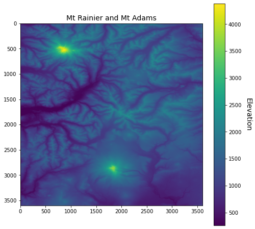
Plot
It’s always useful to plot the data so we know it has been read correctly.
# Plot data
fig, ax = plt.subplots(figsize=(8,8))
im = ax.imshow(elevations)
ax.set_title("Mt Rainier and Mt Adams", fontsize=14)
cbar = fig.colorbar(im, orientation='vertical')
cbar.ax.set_ylabel('Elevation', rotation=270, fontsize=14)
cbar.ax.get_yaxis().labelpad = 20
Sampling the data using points
To sample the raster data at the campsite locations we can use Rasterio's sample function. This function expects a list of x, y coordinate pairs so we need to convert our geometry column using list comprehension.
coord_list = [(x,y) for x,y in zip(campsites['geometry'].x , campsites['geometry'].y)]
coord_list
[(-121.86309568977, 46.9328599291782),
 (-121.644123657629, 46.9024017663544),
 (-121.566675005534, 46.73861426056),
 (-121.794055025156, 46.7676258113237)]
Now we can carry out the sample and store the results in new column called elevation. Note that if the image has more than one band, a value is returned for each band.
campsites['elevation'] = [x for x in src.sample(coord_list)]
campsites.head()
| campsite | lat | lon | geometry | elevation | |
|---|---|---|---|---|---|
| 0 | mowich lake | 46.932860 | -121.863096 | POINT (-121.86310 46.93286) | [1505] |
| 1 | white river | 46.902402 | -121.644124 | POINT (-121.64412 46.90240) | [1331] |
| 2 | ohanapecosh | 46.738614 | -121.566675 | POINT (-121.56668 46.73861) | [609] |
| 3 | cougar rock | 46.767626 | -121.794055 | POINT (-121.79406 46.76763) | [975] |
Buffer points
Sometimes it might be a little risky to sample only one cell per point. There may be errors or artifacts in the unerlying raster. A more robust method would be to sample multiple raster grid cells surrounding a point. To do this we could buffer the points by a set distance and sample the raster values within the buffer.
GeoPandas has a method called buffer which expects a distance around each object. Since our shapefile is in WGS84 coordinate system, this distance would have to be in degrees which is a little confusing. A better option would be to reproject our shapefile into a projected coordinate system so we can enter a buffer distance in meters.
campsites_utm = campsites.to_crs('EPSG:32610')
campsites_utm['buffer'] = campsites_utm.buffer(500)
campsites_utm
| campsite | lat | lon | geometry | elevation | buffer | |
|---|---|---|---|---|---|---|
| 0 | mowich lake | 46.932860 | -121.863096 | POINT (586541.645 5198330.423) | [1505] | POLYGON ((587041.645 5198330.423, 587039.237 5... |
| 1 | white river | 46.902402 | -121.644124 | POINT (603268.211 5195210.763) | [1331] | POLYGON ((603768.211 5195210.763, 603765.804 5... |
| 2 | ohanapecosh | 46.738614 | -121.566675 | POINT (609498.970 5177115.438) | [609] | POLYGON ((609998.970 5177115.438, 609996.562 5... |
| 3 | cougar rock | 46.767626 | -121.794055 | POINT (592078.991 5180047.801) | [975] | POLYGON ((592578.991 5180047.801, 592576.583 5... |
Now we have two columns containing geometry values. But a GeoDataFrame can only have one active geometry. Since we intend to use our buffer geometry to sample the raster data, we will make our buffer column the active geometry.
campsites_utm.set_geometry('buffer', inplace=True)
We have to convert the DataFrame back to WGS84 so it has the same projection system as our raster data.
campsites = campsites_utm.to_crs('EPSG:4326')
Sampling grid cells using polygons
There is a package called rasterstats that makes this task pretty straightforward. In the docs, it recommends installing using pip. We can actually do this directly from a Jupyter Notebook by using the ! mark which allows us execute commands from the underlying operating system.
!pip install rasterstats
Requirement already satisfied: rasterstats in /home/johnny/anaconda3/envs/gds/lib/python3.8/site-packages (0.17.0)
Requirement already satisfied: simplejson in /home/johnny/anaconda3/envs/gds/lib/python3.8/site-packages (from rasterstats) (3.17.6)
Requirement already satisfied: affine<3.0 in /home/johnny/anaconda3/envs/gds/lib/python3.8/site-packages (from rasterstats) (2.3.0)
Requirement already satisfied: fiona in /home/johnny/anaconda3/envs/gds/lib/python3.8/site-packages (from rasterstats) (1.8.20)
Requirement already satisfied: shapely in /home/johnny/anaconda3/envs/gds/lib/python3.8/site-packages (from rasterstats) (1.8.0)
Requirement already satisfied: numpy>=1.9 in /home/johnny/anaconda3/envs/gds/lib/python3.8/site-packages (from rasterstats) (1.22.1)
Requirement already satisfied: cligj>=0.4 in /home/johnny/anaconda3/envs/gds/lib/python3.8/site-packages (from rasterstats) (0.7.2)
Requirement already satisfied: rasterio>=1.0 in /home/johnny/anaconda3/envs/gds/lib/python3.8/site-packages (from rasterstats) (1.2.10)
Requirement already satisfied: click>=4.0 in /home/johnny/anaconda3/envs/gds/lib/python3.8/site-packages (from cligj>=0.4->rasterstats) (8.0.3)
Requirement already satisfied: certifi in /home/johnny/anaconda3/envs/gds/lib/python3.8/site-packages (from rasterio>=1.0->rasterstats) (2022.6.15)
Requirement already satisfied: attrs in /home/johnny/anaconda3/envs/gds/lib/python3.8/site-packages (from rasterio>=1.0->rasterstats) (21.4.0)
Requirement already satisfied: snuggs>=1.4.1 in /home/johnny/anaconda3/envs/gds/lib/python3.8/site-packages (from rasterio>=1.0->rasterstats) (1.4.7)
Requirement already satisfied: setuptools in /home/johnny/anaconda3/envs/gds/lib/python3.8/site-packages (from rasterio>=1.0->rasterstats) (60.5.0)
Requirement already satisfied: click-plugins in /home/johnny/anaconda3/envs/gds/lib/python3.8/site-packages (from rasterio>=1.0->rasterstats) (1.1.1)
Requirement already satisfied: munch in /home/johnny/anaconda3/envs/gds/lib/python3.8/site-packages (from fiona->rasterstats) (2.5.0)
Requirement already satisfied: six>=1.7 in /home/johnny/anaconda3/envs/gds/lib/python3.8/site-packages (from fiona->rasterstats) (1.16.0)
Requirement already satisfied: pyparsing>=2.1.6 in /home/johnny/anaconda3/envs/gds/lib/python3.8/site-packages (from snuggs>=1.4.1->rasterio>=1.0->rasterstats) (3.0.7)
After successfully installing rasterstats, we can go ahead and import the function we need.
from rasterstats import zonal_stats
The zonal_stats function requires a shapefile or polygon, a raster file or array, the geotransform of the array, and the stats we’d like to compute.
stats = zonal_stats(campsites.geometry, elevations, affine=src.transform,
            stats=['mean', 'std', 'count'], nodata=src.nodata)
stats
[{'mean': 1538.70367278798, 'count': 1198, 'std': 61.23086259469099},
 {'mean': 1380.375312760634, 'count': 1199, 'std': 75.87074248803795},
 {'mean': 638.1961602671118, 'count': 1198, 'std': 33.699186100766795},
 {'mean': 1007.7948290241868, 'count': 1199, 'std': 58.850863432257526}]
The mean value provides a robust measure of elevation surrounding each campsite. By including the count option we can see that there were 1198/1199 grid cells sampled for each 500 m buffer. The std option provides the variance of elevations in the buffer.
We can add these data to our original GeoDataFrame. Luckily for us, Pandas can implicitly convert a list of dictionaries to a DataFrame. Since zonal_stats preserves the order of campsites, we can use the index to merge the two DataFrames.
campsite_stats = campsites.merge(pd.DataFrame(stats), left_index=True, right_index=True)
campsite_stats
| campsite | lat | lon | geometry | elevation | buffer | mean | count | std | median | |
|---|---|---|---|---|---|---|---|---|---|---|
| 0 | mowich lake | 46.932860 | -121.863096 | POINT (586541.645 5198330.423) | [1505] | POLYGON ((-121.85653 46.93279, -121.85657 46.9... | 1538.703673 | 1198 | 61.230863 | 1527.0 |
| 1 | white river | 46.902402 | -121.644124 | POINT (603268.211 5195210.763) | [1331] | POLYGON ((-121.63756 46.90232, -121.63760 46.9... | 1380.375313 | 1199 | 75.870742 | 1353.0 |
| 2 | ohanapecosh | 46.738614 | -121.566675 | POINT (609498.970 5177115.438) | [609] | POLYGON ((-121.56013 46.73853, -121.56018 46.7... | 638.196160 | 1198 | 33.699186 | 632.0 |
| 3 | cougar rock | 46.767626 | -121.794055 | POINT (592078.991 5180047.801) | [975] | POLYGON ((-121.78751 46.76756, -121.78755 46.7... | 1007.794829 | 1199 | 58.850863 | 986.0 |