Vector data analysis
Contents
Vector data analysis
The vector data model represents features on the Earth’s surface as points, lines or polygons. Vector data is useful for storing and representing data that has discrete boundaries, such as borders, buildings, streets, and roads. Online mapping applications, such as Google Maps and OpenStreetMap, use this format to display data.
The Python library GeoPandas provides somes great tools for working with vector data. As the name suggests, GeoPandas extends the popular data science library Pandas by adding support for geospatial data. The core data structure in GeoPandas is the GeoDataFrame. The key difference between the two is that a GeoDataFrame can store geometry data and perform spatial operations.

The geometry column can contain any geometry type (e.g. points, lines, polygons) or even a mixture.
Reading files
Assuming we have a file containing both data and geometry (e.g. GeoPackage, GeoJSON, Shapefile), we can read it using read_file(), which automatically detects the filetype and creates a GeoDataFrame. In the this demo, we will be working with a shapefile that contains the states of the contiguous United States.
import geopandas as gpd

gdf = gpd.read_file('data/us_states.shp')
gdf.head()
| STATEFP | STUSPS | NAME | geometry | |
|---|---|---|---|---|
| 0 | 24 | MD | Maryland | MULTIPOLYGON (((1722285.499 1847164.899, 17253... |
| 1 | 19 | IA | Iowa | POLYGON ((-50588.826 2198204.224, -46981.682 2... |
| 2 | 10 | DE | Delaware | POLYGON ((1705277.992 2038007.044, 1706136.968... |
| 3 | 39 | OH | Ohio | MULTIPOLYGON (((1081987.294 2151544.264, 10846... |
| 4 | 42 | PA | Pennsylvania | POLYGON ((1287711.752 2093650.229, 1286266.040... |
type(gdf)
geopandas.geodataframe.GeoDataFrame
Note
The geometry column is the active geometry. Spatial methods used on the GeoDataFrame will use these geometries.
Geometric properties
Since we have a GeoDataFrame that is spatially “aware”, we can compute the geometric properties for each row. For example, we could make a new column that contains the area of each state:
gdf['area'] = gdf['geometry'].area
gdf.head()
| STATEFP | STUSPS | NAME | geometry | area | |
|---|---|---|---|---|---|
| 0 | 24 | MD | Maryland | MULTIPOLYGON (((1722285.499 1847164.899, 17253... | 2.754245e+10 |
| 1 | 19 | IA | Iowa | POLYGON ((-50588.826 2198204.224, -46981.682 2... | 1.456667e+11 |
| 2 | 10 | DE | Delaware | POLYGON ((1705277.992 2038007.044, 1706136.968... | 5.324652e+09 |
| 3 | 39 | OH | Ohio | MULTIPOLYGON (((1081987.294 2151544.264, 10846... | 1.069777e+11 |
| 4 | 42 | PA | Pennsylvania | POLYGON ((1287711.752 2093650.229, 1286266.040... | 1.173572e+11 |
Or the centroid of each state
gdf['centroid'] = gdf['geometry'].centroid
gdf.head()
| STATEFP | STUSPS | NAME | geometry | area | centroid | |
|---|---|---|---|---|---|---|
| 0 | 24 | MD | Maryland | MULTIPOLYGON (((1722285.499 1847164.899, 17253... | 2.754245e+10 | POINT (1640385.402 1944865.873) |
| 1 | 19 | IA | Iowa | POLYGON ((-50588.826 2198204.224, -46981.682 2... | 1.456667e+11 | POINT (205832.463 2121901.888) |
| 2 | 10 | DE | Delaware | POLYGON ((1705277.992 2038007.044, 1706136.968... | 5.324652e+09 | POINT (1745372.416 1963739.545) |
| 3 | 39 | OH | Ohio | MULTIPOLYGON (((1081987.294 2151544.264, 10846... | 1.069777e+11 | POINT (1109302.074 1996734.113) |
| 4 | 42 | PA | Pennsylvania | POLYGON ((1287711.752 2093650.229, 1286266.040... | 1.173572e+11 | POINT (1512084.467 2130516.771) |
Plot
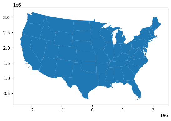
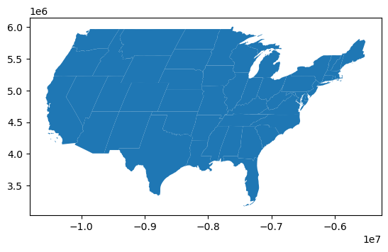
We can use plot() to produce a basic vizualisation of the geometries.
gdf.plot()
<Axes: >
We can also explore our data interactively using GeoDataFrame.explore(), which behaves in the same way plot() does but returns an interactive map instead.
gdf.explore()
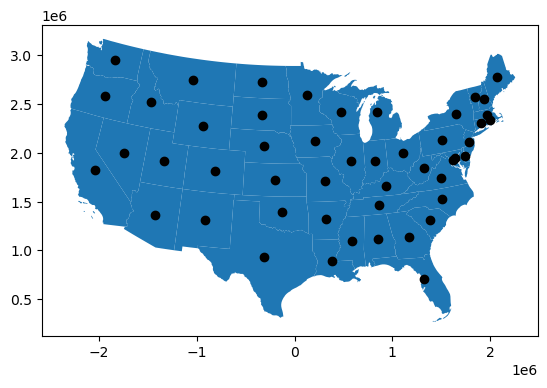
Finally, we can plot two geometry columns together, we just need to use one plot as an axis for the other.
ax = gdf['geometry'].plot()
gdf['centroid'].plot(ax=ax, color='black')
<Axes: >
Indexing
GeoPandas inherits the standard Pandas methods for indexing/selecting data. We can use integer position based indexing (iloc) to select rows:
gdf.iloc[3:6]
| STATEFP | STUSPS | NAME | geometry | area | centroid | |
|---|---|---|---|---|---|---|
| 3 | 39 | OH | Ohio | MULTIPOLYGON (((1081987.294 2151544.264, 10846... | 1.069777e+11 | POINT (1109302.074 1996734.113) |
| 4 | 42 | PA | Pennsylvania | POLYGON ((1287711.752 2093650.229, 1286266.040... | 1.173572e+11 | POINT (1512084.467 2130516.771) |
| 5 | 31 | NE | Nebraska | POLYGON ((-670097.365 2040215.635, -668488.696... | 2.003646e+11 | POINT (-314201.847 2065223.842) |
gdf.iloc[30]
STATEFP                                                    32
STUSPS                                                     NV
NAME                                                   Nevada
geometry    POLYGON ((-2028959.4341761633 2068002.78284196...
area                                      286343437541.051636
centroid         POINT (-1748436.870197715 2002314.685556594)
Name: 30, dtype: object
It is also possible to select a subset of data based on a mask, with the syntax df[df['column_name'] == 'some value']. This operation selects only the rows where this condition is true:
gdf[gdf['NAME'] == 'Oregon']
| STATEFP | STUSPS | NAME | geometry | area | centroid | |
|---|---|---|---|---|---|---|
| 15 | 41 | OR | Oregon | POLYGON ((-2285910.272 2550894.134, -2276699.4... | 2.513754e+11 | POINT (-1943081.490 2579189.994) |
Sometimes we might want to select rows where a column value is in list of values
western_states = ['Oregon', 'Washington', 'California']
gdf[gdf['NAME'].isin(western_states)]
| STATEFP | STUSPS | NAME | geometry | area | centroid | |
|---|---|---|---|---|---|---|
| 6 | 53 | WA | Washington | MULTIPOLYGON (((-2000237.694 3142051.285, -198... | 1.788164e+11 | POINT (-1840167.993 2949083.273) |
| 11 | 06 | CA | California | MULTIPOLYGON (((-2066284.899 1402243.639, -205... | 4.105166e+11 | POINT (-2043435.932 1824815.053) |
| 15 | 41 | OR | Oregon | POLYGON ((-2285910.272 2550894.134, -2276699.4... | 2.513754e+11 | POINT (-1943081.490 2579189.994) |
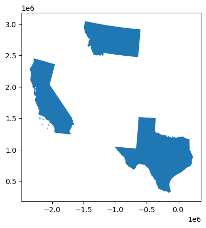
# Select all states with an area larger than 3.5e+11 m2
gdf[gdf['area'] > 3.5e+11]
| STATEFP | STUSPS | NAME | geometry | area | centroid | |
|---|---|---|---|---|---|---|
| 10 | 48 | TX | Texas | POLYGON ((-998043.807 1038046.289, -997956.109... | 6.926631e+11 | POINT (-312496.251 936222.085) |
| 11 | 06 | CA | California | MULTIPOLYGON (((-2066284.899 1402243.639, -205... | 4.105166e+11 | POINT (-2043435.932 1824815.053) |
| 25 | 30 | MT | Montana | POLYGON ((-1474367.320 3044425.629, -1434636.1... | 3.806067e+11 | POINT (-1037341.467 2747065.255) |
# Plot all states with an area larger than 2.5e+11 m2
gdf[gdf['area'] > 3.5e+11].plot()
<Axes: >
Projections
GeoDataFrames have their own Coordinate Reference System (CRS) which can be accessed using the crs method. The CRS tells GeoPandas where the coordinates of the geometries are located on the Earth’s surface. If we run this on our data, we will see that it has an Albers Equal Area projection.
gdf.crs
<Projected CRS: EPSG:5070>
Name: NAD83 / Conus Albers
Axis Info [cartesian]:
- X[east]: Easting (metre)
- Y[north]: Northing (metre)
Area of Use:
- name: United States (USA) - CONUS onshore - Alabama; Arizona; Arkansas; California; Colorado; Connecticut; Delaware; Florida; Georgia; Idaho; Illinois; Indiana; Iowa; Kansas; Kentucky; Louisiana; Maine; Maryland; Massachusetts; Michigan; Minnesota; Mississippi; Missouri; Montana; Nebraska; Nevada; New Hampshire; New Jersey; New Mexico; New York; North Carolina; North Dakota; Ohio; Oklahoma; Oregon; Pennsylvania; Rhode Island; South Carolina; South Dakota; Tennessee; Texas; Utah; Vermont; Virginia; Washington; West Virginia; Wisconsin; Wyoming.
- bounds: (-124.79, 24.41, -66.91, 49.38)
Coordinate Operation:
- name: Conus Albers
- method: Albers Equal Area
Datum: North American Datum 1983
- Ellipsoid: GRS 1980
- Prime Meridian: Greenwich
We can reproject a our data using the to_crs method.
gdf_reproject = gdf.to_crs('EPSG:4326')
gdf_reproject.crs
<Geographic 2D CRS: EPSG:4326>
Name: WGS 84
Axis Info [ellipsoidal]:
- Lat[north]: Geodetic latitude (degree)
- Lon[east]: Geodetic longitude (degree)
Area of Use:
- name: World.
- bounds: (-180.0, -90.0, 180.0, 90.0)
Datum: World Geodetic System 1984 ensemble
- Ellipsoid: WGS 84
- Prime Meridian: Greenwich
Tip
It is recommended to use an EPSG code for specifying projections. We can find the right EPSG code using this site: https://epsg.io/
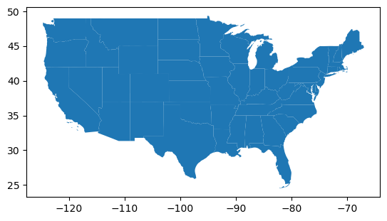
Now we will see that our geometry column contains longitudes and latitudes (i.e. in degrees). It also looks a bit different when we plot it (also note the x- y-axis scales).
gdf_reproject.head()
| STATEFP | STUSPS | NAME | geometry | area | centroid | |
|---|---|---|---|---|---|---|
| 0 | 24 | MD | Maryland | MULTIPOLYGON (((-76.04621 38.02553, -76.00733 ... | 2.754245e+10 | POINT (1640385.402 1944865.873) |
| 1 | 19 | IA | Iowa | POLYGON ((-96.62188 42.77925, -96.57794 42.827... | 1.456667e+11 | POINT (205832.463 2121901.888) |
| 2 | 10 | DE | Delaware | POLYGON ((-75.77378 39.72220, -75.75323 39.757... | 5.324652e+09 | POINT (1745372.416 1963739.545) |
| 3 | 39 | OH | Ohio | MULTIPOLYGON (((-82.86334 41.69369, -82.82571 ... | 1.069777e+11 | POINT (1109302.074 1996734.113) |
| 4 | 42 | PA | Pennsylvania | POLYGON ((-80.51989 40.90666, -80.51964 40.987... | 1.173572e+11 | POINT (1512084.467 2130516.771) |
gdf_reproject.plot()
<Axes: >
Note
Sometimes GeoPandas won’t recognize the EPSG code. In this case, we can navigate to epsg.io and use the projection description to reproject the data. If there isn’t a description, scroll down to PROJ.4 in the Export menu and copy and paste from there.
# Reproject to World Eckert IV (https://epsg.io/54012)
proj = '+proj=eck4 +lon_0=0 +x_0=0 +y_0=0 +ellps=WGS84 +datum=WGS84 +units=m no_defs'
gdf_reproject = gdf_reproject.to_crs(proj)
gdf_reproject.plot()
<Axes: >
Writing files
We can write a GeoDataFrame back to file using GeoDataFrame.to_file(). The default file format is a shapefile. Note that we can only have one geometry column so we drop the centroid column before writing.
gdf_reproject.drop(columns=['centroid']).to_file('data/us_states_wgs84.shp')