More vector data analysis¶

In the second demo of this week, we will introduce the basics of vector data analysis in Python with an example. We have two shapefiles. The first shapefile contains the name, location, and capacity of all major sports stadiums in the United States as points. The second shapefile contains the states on the United States as polygons. An alien would like to know which state contains the highest number of stadiums, the highest number of seats, and the closest and furthest stadiums from University of Oregon’s campus.

import geopandas as gpd

# Import data
stadiums = gpd.read_file('data/sports_venues.shp')
states = gpd.read_file('data/us_states.shp')

stadiums

	NAME	CAPACITY	geometry
0	MILWAUKEE MILE	45000.0	POINT (-9797298.508 5315043.944)
1	STREETS OF ST. PETERSBURG	-999.0	POINT (-9198320.620 3219439.478)
2	STREETS OF LONG BEACH	-999.0	POINT (-13157142.784 3997054.057)
3	BARBER MOTORSPORTS PARK	-999.0	POINT (-9642382.973 3966132.844)
4	STREETS OF TORONTO	-999.0	POINT (-8840529.757 5408873.389)
...	...	...	...
819	UPMC EVENTS CENTER	4000.0	POINT (-8929463.890 4941833.552)
820	GLOBE LIFE FIELD	40000.0	POINT (-10807587.284 3861421.677)
821	WEATHERTECH RACEWAY LAGUNA SECA	11000.0	POINT (-13553512.291 4381243.369)
822	CIRCUIT OF THE AMERICAS	120000.0	POINT (-10868589.591 3520977.940)
823	LAS VEGAS STADIUM	65000.0	POINT (-12822172.352 4313213.054)

824 rows × 3 columns

Explore¶

It is always good practice to start with a visualization to check everything is projected properly.

stadiums.explore()

Make this Notebook Trusted to load map: File -> Trust Notebook

stadiums.info()

<class 'geopandas.geodataframe.GeoDataFrame'>
RangeIndex: 824 entries, 0 to 823
Data columns (total 3 columns):
 #   Column    Non-Null Count  Dtype   
---  ------    --------------  -----   
 0   NAME      824 non-null    object  
 1   CAPACITY  824 non-null    float64 
 2   geometry  824 non-null    geometry
dtypes: float64(1), geometry(1), object(1)
memory usage: 19.4+ KB

The info() method reveals that there are no missing values… or are there?

stadiums.describe()

	CAPACITY
count	824.000000
mean	20984.593447
std	26260.948903
min	-999.000000
25%	4584.500000
50%	10333.500000
75%	26436.000000
max	257325.000000

Remove missing values¶

When we run describe() we notice that the min value is -999 which is a value often used to indicate no data. Since we have no logical way of interpolating those values, we will just remove these rows. We can do this by filtring our DataFrame with a mask that returns True if values are not equal to -999.

stadiums = stadiums[stadiums['CAPACITY'] != -999]
stadiums.describe()

	CAPACITY
count	722.000000
mean	24090.308864
std	26630.288096
min	837.000000
25%	6500.000000
50%	13073.000000
75%	31875.000000
max	257325.000000

Check projections¶

If we are going to find how many stadiums are in each state, we will need to join the DataFrames. But we can only do this if they are in the same projection.

stadiums.crs

<Derived Projected CRS: EPSG:3857>
Name: WGS 84 / Pseudo-Mercator
Axis Info [cartesian]:
- X[east]: Easting (metre)
- Y[north]: Northing (metre)
Area of Use:
- name: World between 85.06°S and 85.06°N.
- bounds: (-180.0, -85.06, 180.0, 85.06)
Coordinate Operation:
- name: Popular Visualisation Pseudo-Mercator
- method: Popular Visualisation Pseudo Mercator
Datum: World Geodetic System 1984 ensemble
- Ellipsoid: WGS 84
- Prime Meridian: Greenwich

states.crs

<Derived Projected CRS: EPSG:5070>
Name: NAD83 / Conus Albers
Axis Info [cartesian]:
- X[east]: Easting (metre)
- Y[north]: Northing (metre)
Area of Use:
- name: United States (USA) - CONUS onshore - Alabama; Arizona; Arkansas; California; Colorado; Connecticut; Delaware; Florida; Georgia; Idaho; Illinois; Indiana; Iowa; Kansas; Kentucky; Louisiana; Maine; Maryland; Massachusetts; Michigan; Minnesota; Mississippi; Missouri; Montana; Nebraska; Nevada; New Hampshire; New Jersey; New Mexico; New York; North Carolina; North Dakota; Ohio; Oklahoma; Oregon; Pennsylvania; Rhode Island; South Carolina; South Dakota; Tennessee; Texas; Utah; Vermont; Virginia; Washington; West Virginia; Wisconsin; Wyoming.
- bounds: (-124.79, 24.41, -66.91, 49.38)
Coordinate Operation:
- name: Conus Albers
- method: Albers Equal Area
Datum: North American Datum 1983
- Ellipsoid: GRS 1980
- Prime Meridian: Greenwich

Since they are in different projections, we will convert the stadiums DataFrame to match the states DataFrame.

stadiums = stadiums.to_crs('EPSG:5070')
stadiums.crs

<Derived Projected CRS: EPSG:5070>
Name: NAD83 / Conus Albers
Axis Info [cartesian]:
- X[east]: Easting (metre)
- Y[north]: Northing (metre)
Area of Use:
- name: United States (USA) - CONUS onshore - Alabama; Arizona; Arkansas; California; Colorado; Connecticut; Delaware; Florida; Georgia; Idaho; Illinois; Indiana; Iowa; Kansas; Kentucky; Louisiana; Maine; Maryland; Massachusetts; Michigan; Minnesota; Mississippi; Missouri; Montana; Nebraska; Nevada; New Hampshire; New Jersey; New Mexico; New York; North Carolina; North Dakota; Ohio; Oklahoma; Oregon; Pennsylvania; Rhode Island; South Carolina; South Dakota; Tennessee; Texas; Utah; Vermont; Virginia; Washington; West Virginia; Wisconsin; Wyoming.
- bounds: (-124.79, 24.41, -66.91, 49.38)
Coordinate Operation:
- name: Conus Albers
- method: Albers Equal Area
Datum: North American Datum 1983
- Ellipsoid: GRS 1980
- Prime Meridian: Greenwich

Join DataFrames¶

A spatial join (sjoin) can be used to combine two GeoDataFrames based on the spatial relationship between their geometries. A common use case might be a spatial join between a point layer (stadiums) and a polygon layer (states) so that we we retain the point geometries and add the attributes of the intersecting polygons.

Now we know from exploring the data that there are some stadiums that are outside the US. We would like to exclude those from our analysis. An inner join (how='inner'), keeps rows from both GeoDataFrames only when the points are contained within the polygons.

stadiums_usa = stadiums.sjoin(states, how='inner')

Now when we plot our data again, we find that there are no stadiums outside the USA and that the points have more attributes, including the state that they are within.

stadiums_usa.explore()

Make this Notebook Trusted to load map: File -> Trust Notebook

Compute stats¶

We can complete our first task by grouping the stadiums by state, summing their capacities, and sorting from highest to lowest.

stadiums_usa.groupby('NAME_right')['CAPACITY'].sum().sort_values(ascending=False).head()

NAME_right
Texas         1493214.0
California    1383573.0
Florida        987111.0
Indiana        675805.0
Ohio           641793.0
Name: CAPACITY, dtype: float64

Note

Calling more than one method on an object is called method chaining.

top_state = stadiums_usa.groupby('NAME_right')['CAPACITY'].sum().sort_values(ascending=False).index[0]
top_seats = stadiums_usa.groupby('NAME_right')['CAPACITY'].sum().sort_values(ascending=False).iloc[0]

f"{top_state} has the most stadium seats in the US with {int(top_seats)}"

'Texas has the most stadium seats in the US with 1493214'

If we wanted to find the state with the most stadiums we could can just change sum() to count().

stadiums_usa.groupby('NAME_right')['CAPACITY'].count().sort_values(ascending=False).head()

NAME_right
California        58
Texas             52
New York          39
Florida           33
North Carolina    30
Name: CAPACITY, dtype: int64

top_state = stadiums_usa.groupby('NAME_right')['CAPACITY'].count().sort_values(ascending=False).index[0]
top_stadiums = stadiums_usa.groupby('NAME_right')['CAPACITY'].count().sort_values(ascending=False).iloc[0]

f"{top_state} has the most sports stadiums in the US with {int(top_stadiums)}"

'California has the most sports stadiums in the US with 58'

Measure distance¶

Our final task is to compute the distance between University of Oregon campus and all the stadiums in the dataset.

Caution

When computing distance or area, we must ensure that our data have a projected CRS (in meters, feet, kilometers etc.), eather than geographic CRS (in degrees).

We are OK to compute distances using our stadium data because when we call the crs method, we can see that the Easting and Northing are in the meters.

stadiums_usa.crs

<Derived Projected CRS: EPSG:5070>
Name: NAD83 / Conus Albers
Axis Info [cartesian]:
- X[east]: Easting (metre)
- Y[north]: Northing (metre)
Area of Use:
- name: United States (USA) - CONUS onshore - Alabama; Arizona; Arkansas; California; Colorado; Connecticut; Delaware; Florida; Georgia; Idaho; Illinois; Indiana; Iowa; Kansas; Kentucky; Louisiana; Maine; Maryland; Massachusetts; Michigan; Minnesota; Mississippi; Missouri; Montana; Nebraska; Nevada; New Hampshire; New Jersey; New Mexico; New York; North Carolina; North Dakota; Ohio; Oklahoma; Oregon; Pennsylvania; Rhode Island; South Carolina; South Dakota; Tennessee; Texas; Utah; Vermont; Virginia; Washington; West Virginia; Wisconsin; Wyoming.
- bounds: (-124.79, 24.41, -66.91, 49.38)
Coordinate Operation:
- name: Conus Albers
- method: Albers Equal Area
Datum: North American Datum 1983
- Ellipsoid: GRS 1980
- Prime Meridian: Greenwich

We will first create a GeoDataFrame with a single row that represents the longitude and latitude of campus (-123.0783, 44.04505) as a Point data type.

from shapely.geometry import Point

data = {'geometry': [Point(-123.0783, 44.04505)]}

s = gpd.GeoDataFrame(data, crs="EPSG:4326")
s

	geometry
0	POINT (-123.07830 44.04505)

Next we must convert this GeoDataFrame to the same projection as our stadium data (EPSG:5070).

s.to_crs('EPSG:5070', inplace=True)
s

	geometry
0	POINT (-2133399.001 2645357.154)

Now we can compute distances to all stadiums in the United States using the distance() method.

distance = stadiums_usa.distance(s['geometry'].iloc[0])
distance 

    2.807969e+06
   2.771818e+06
  2.695892e+06
  2.810889e+06
  2.790744e+06
           ...     
  2.072308e+06
  2.056440e+06
  2.089632e+06
  2.105634e+06
  2.105656e+06
Length: 696, dtype: float64

Let’s add this new data as a column to our original GeoDataFrame and convert to kilometers.

stadiums_usa['distance_to_eugene'] = distance / 1000
stadiums_usa

	NAME_left	CAPACITY	geometry	index_right	STATEFP	STUSPS	NAME_right	distance_to_eugene
0	MILWAUKEE MILE	45000.0	POINT (646905.219 2252165.087)	14	55	WI	Wisconsin	2807.969295
46	LAMBEAU FIELD	81441.0	POINT (628952.471 2416474.808)	14	55	WI	Wisconsin	2771.817595
155	CAMP RANDALL STADIUM	80321.0	POINT (533197.371 2249000.861)	14	55	WI	Wisconsin	2695.892157
189	MILLER PARK	41900.0	POINT (650017.078 2253318.084)	14	55	WI	Wisconsin	2810.889486
274	ROAD AMERICA	40000.0	POINT (640442.284 2338673.449)	14	55	WI	Wisconsin	2790.743695
...	...	...	...	...	...	...	...	...
483	SCHEELS CENTER	5830.0	POINT (-61123.759 2656923.016)	37	38	ND	North Dakota	2072.307518
648	BETTY ENGELSTAD SIOUX CENTER	3300.0	POINT (-80779.004 2770637.937)	37	38	ND	North Dakota	2056.439673
484	FROST ARENA	6500.0	POINT (-61986.213 2370021.948)	41	46	SD	South Dakota	2089.631646
658	DAKOTADOME	10000.0	POINT (-75459.148 2199735.337)	41	46	SD	South Dakota	2105.634167
776	SANFORD COYOTE SPORTS CENTER	6000.0	POINT (-75464.732 2199604.063)	41	46	SD	South Dakota	2105.656495

696 rows × 8 columns

Make a map¶

We can plot the stadium data again but this time using time color the dots based on distance to campus. See here for more examples of interactive plotting and here for a full list of colormaps.

stadiums_usa.explore(column='distance_to_eugene', cmap='Set1')

Make this Notebook Trusted to load map: File -> Trust Notebook

Note

The explore() method returns a folium.Map object which is a really nice way of making interactive maps. We don’t have enough time to cover Folium in this course. But we use it a lot in Geospatial Data Science, the next course in this series.

Choropleth maps¶

Choropleth maps, where the color of each shape is based on the value of an associated variable, are a useful for displaying geospatial data. If we wanted to produce a chloropleth map showing the number of stadiums in each state, we would first group the stadium data by state.

stadiums_by_state = stadiums_usa.groupby('NAME_right')['CAPACITY'].count().reset_index()
stadiums_by_state.head()

	NAME_right	CAPACITY
0	Alabama	16
1	Arizona	11
2	Arkansas	9
3	California	58
4	Colorado	13

Then we would join this new dataframe with the original GeoDataFrame of US states so we can add the geometry data. This time we are joining based on a primary key which has to be specified using the left_on and right_on keyword arguments.

states_merge = states.merge(stadiums_by_state, left_on='NAME', right_on='NAME_right')
states_merge.head()

	STATEFP	STUSPS	NAME	geometry	NAME_right	CAPACITY
0	24	MD	Maryland	MULTIPOLYGON (((1722285.499 1847164.899, 17253...	Maryland	16
1	19	IA	Iowa	POLYGON ((-50588.826 2198204.224, -46981.682 2...	Iowa	8
2	10	DE	Delaware	POLYGON ((1705277.992 2038007.044, 1706136.968...	Delaware	3
3	39	OH	Ohio	MULTIPOLYGON (((1081987.294 2151544.264, 10846...	Ohio	30
4	42	PA	Pennsylvania	POLYGON ((1287711.752 2093650.229, 1286266.040...	Pennsylvania	25

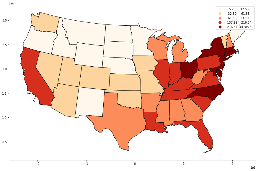
Now we can make our chloropleth map but first let’s compute another variable: stadium density.

states_merge['area'] = states_merge.area / 1000000000000
states_merge['stadium_density'] = states_merge['CAPACITY'] / states_merge['area'] 

states_merge.plot(
    column="stadium_density",
    cmap='OrRd',
    legend=True,
    scheme="quantiles",
    edgecolor='black',
    figsize=(15, 10))

<AxesSubplot:>

Programming for spatial data science

More vector data analysis

Contents

More vector data analysis¶

Explore¶

Remove missing values¶

Check projections¶

Join DataFrames¶

Compute stats¶

Measure distance¶

Make a map¶

Choropleth maps¶